by Bogumil Kaminski
Warmup #1
How to calculate a mean(or histogram or ..., including writing) of 2 000 000 000 floats on a laptop with 8GB RAM?
What is the problem one float is one 8 bytes so actually this data set is much larger than my RAM
@time s = SharedArray{Float64}("/Users/Wucutin/Desktop/Julia/test.bin", (2*10^9,)) # map it to a file
typeof(s)
size(s)
# read data and swap between memory and hard drive
@time println(mean(s))
Warmup #1 reloaded
Now handle (standard filters, maps, joins,...) 1600 homogenous CSVs, 10MB each containing high-frequency trading data (using all your cores, the same laptop)
JuliaDB
Warmup #2
Run bootstrapping on all your cores with shared memory between processes
bootstrapping can parallize very well, because you can actually every iteration of bootstrapping can be done independently. The probelm with bootstrapping starts if I want to distributed among many cores that actually are know for example in R you would have to copy the same data onto every process. If I have large volum data, I'll run out of RAM
# start: julia -p auto
addprocs(4)
nworkers()
s = SharedArray{Float64}((10^5, )); s .= rand(10^5);
@everywhere f(x) = [mean(rand(x, length(x))) for i in 1:1000]
# bootstrap1 run on one core, standard bootstrapping procedurem
function f1(x)
    var(vcat([f(x) for i in 1:4]...))
end
# bootstrap2 distribute all the cores I have
function f2(x)
    ps = [@spawn f(x) for i in 1:4]
    var(vcat([fetch(p) for p in ps]...))
end
@time f1(s)
@time f2(s)
Warmup #3
Read 15.17MB text data encoded in UTF-8
String memory footprint in bytes:
- Julia: 15 912 000
- Python: 29 172 074
Asian option pricing (1)
An asset with known price $X_0$ at time 0
By $X_t$ denote asset price at time t
We have to calculate value v of Asian option executable at time T:
$$v = E[exp(-rT)max(\bar X - K, 0)]$$ $$where \bar X = \frac{1}{T} \int_0^T X_t dt$$
Asian option pricing (2)
Here a standard approach would be use geometric Brownian motion to simulate the move of the stock price and then this is the recursive formula for the price of the stock,
Replace $\bar X$ by its approximation in m discrete periods $$\hat{x} = \frac{1}{m} \sum_{i=1}^m X_{i\Delta}, \Delta = T/m$$
Assume that process $x_t$ is GBM with drift $r$ and volatility $\sigma^2$ $$X_{(i+1)\Delta} = X_{i\Delta} exp \left( \left( r - \frac{\sigma^2}{2} \right) \Delta + \sigma \sqrt{\Delta} Z_i \right ), Z_i \sim N(0,1)$$
Average $n$ independent samples of $exp(-rT)max(\hat{x} - K, 0)$
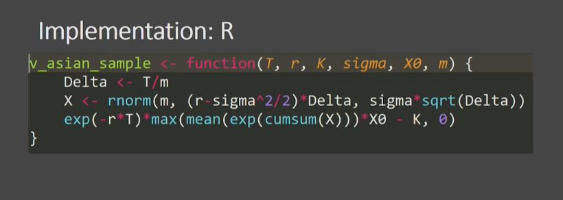
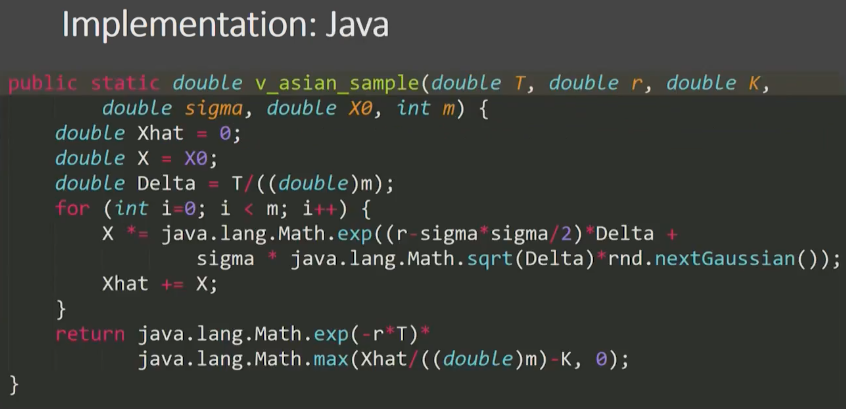
Implementation: Julia
# Method 1
function v_asian_sample(T, r, K, σ, X₀, m)
    x̂ = 0.0
    X::Float64 = X₀
    Δ = T/m
    for i in 1:m
        X *= exp((r - σ^2/2)*Δ + σ*√Δ*randn())
        x̂ += X
    end
    exp(-r*T) * max(x̂/m - K, 0)
end
# Method 2, like the implementation in R
function v_asian_sample2(T, r, K, σ, X₀, m)
    Δ = T/m
    X = σ*√Δ*randn(m) .+ (r - σ^2/2)*Δ
    exp(-r * T) * max(mean(exp.(cumsum!(X, X))) * X₀ - K, 0)
end
Implementation: Python
import math
import random
from numba import jit

@jit
def v_asian_sample(T, r, K, s, X0, m):
    xhat = 0.0
    X = X0
    D = T/m
    for i in range(m):
        X *= math.exp(random.normalvariate((r - s**2/2)*D, s*D**0.5))
        xhat += X
        return math.exp(-r*T)*max(xhat/m - K, 0)